ParametricManager

Similar to the ProjectManager, ORIBT provides the ParametricManager to run simple parametric studies by defining a subset of the inputs as a list. This allows for tradeoff studies to compare the effects of siting (e.g., water depth and distance) on cost and installation timing. For complete details on using the ParametricManager please see the API documentation.

First, we'll import the necessary libraries, and load the example fixed-bottom project to use as our project base with the 15 MW turbine.

from pathlib import Path

import pandas as pd
import matplotlib.pyplot as plt
from matplotlib.ticker import StrMethodFormatter

from ORBIT import ParametricManager, load_config

here = Path(".").resolve()
match here.stem:
    case "examples":
        example_dir = here
    case "tutorials":
        example_dir = here.parents[1] / "examples"
    case "ORBIT":
        example_dir = here / "examples"
    case _:
        msg = "Please manually change `example_dir` if running in a custom location."
        raise FileNotFoundError(msg)

config = load_config(example_dir / "configs/example_fixed_project.yaml")
config["turbine"] = "15MW_generic"

weather = pd.read_csv(example_dir / "data/example_weather.csv").set_index("datetime")

Setting Up The Parameterized Inputs

For all the non-parameterized inputs, they can be left as-is. However, all parameterized variables should be provided in a separate dictionary as a list. Because ORBIT uses the benedict library for more streamlined dictionary access, nested keys can be represented using dot-notation as is shown below where we parameterize the key siting details.

params = {
   "site.depth": list(range(10, 71, 10)),
   "site.distance": list(range(20, 201, 20)),
}

Similar to the parameterized inputs, we must also define the desired outputs. However, outputs must be provided as a dictionary of lambda functions for what metrics should be captured. In the below example, we extract just the installation and system CapEx.

results = {
   "Installation": lambda project: project.installation_capex,
   "System": lambda project: project.system_capex
}

Previewing and Running The Model

If many parameters are configured, it will take a longer time to run, especially if a weather profile is provided and product=True. To get an idea of the total run time, use the preview method, as seen below.

Setting product to True means that all of the parameters will be run as a combination of all possible permutations rather than a zipped list. When using False extra care must be taken to ensure the correct outcomes will be achieved by using equally-lengthed parameterizations. For instance, in our current example, the shortest parameterization has only 3 values, so the first 3 values of depth and distance will be selected for the parameterized run.

project = ParametricManager(config, params, results, product=True, weather=weather)
project.preview()

ORBIT library intialized at '/opt/hostedtoolcache/Python/3.13.13/x64/lib/python3.13/site-packages/library'
10 runs elapsed time: 7.72s
70 runs estimated time: 54.02s

	site.depth	site.distance	Installation	System
0	10	140	3.348771e+08	1.008934e+09
1	60	200	3.751880e+08	1.294177e+09
2	30	200	3.501844e+08	1.116196e+09
3	60	40	3.189682e+08	1.294177e+09
4	10	120	3.303689e+08	1.008934e+09
5	30	100	3.305695e+08	1.116196e+09
6	50	100	3.361646e+08	1.232635e+09
7	20	160	3.428775e+08	1.061392e+09
8	50	180	3.615505e+08	1.232635e+09
9	30	80	3.271180e+08	1.116196e+09

project.run()

The results are saved as a pandas DataFrame in the results attribute where each row represents a different scenario run and the columns are labeled with with the various parameters and results values that were configured.

Plotting The Results

It is more convenient to plot the results of the ParametricManager than it is to view them as a table, especially with a large number of parameters. First, we will create a matrix of results for each of the installation and system CapEx. Please note the installation_arr index is sorted in reverse order for convenience in creating the heatmap.

results = project.results.set_index(["site.depth", "site.distance"]) / 1e6
installation_arr = results.unstack()["Installation"].sort_index(ascending=False)
system_arr = results.unstack()["System"].sort_index()

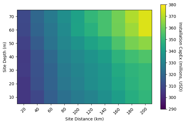
As mentioned in the ProjectManager tutorial, the system CapEx will not change given certain parameter changes. In this case, the installation CapEx increases both as the site's distance and depth increases, as can be seen in the following heatmap.

fig = plt.figure()
ax = fig.add_subplot(111)

im = ax.imshow(installation_arr.values, vmin=290, vmax=380)

cbar = fig.colorbar(im, ax=ax, shrink=0.8)
cbar.ax.set_ylabel("Installation CapEx (millions, USD)", rotation=-90, va="bottom")

ax.set_xticks(
    range(len(installation_arr.columns)),
    labels=installation_arr.columns,
    rotation=45,
    ha="right",
    rotation_mode="anchor"
)
ax.set_yticks(range(len(installation_arr.index)), labels=installation_arr.index)

ax.set_xlabel("Site Distance (km)")
ax.set_ylabel("Site Depth (m)")

fig.tight_layout()

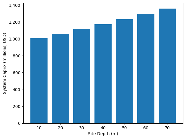
The system CapEx in this example does not change with site distance. The increase in system CapEx with depth can be seen in the bar graph below.

fig = plt.figure()
ax = fig.add_subplot(111)

x = range(len(system_arr.index))
ax.bar(x, system_arr.values[:, 0])

ax.set_xticks(x)
ax.set_xticklabels(system_arr.index.values)
ax.yaxis.set_major_formatter(StrMethodFormatter("{x:,.0f}"))
ax.set_xlabel("Site Depth (m)")
ax.set_ylabel("System CapEx (millions, USD)")

fig.tight_layout()