Custom Array Cabling Guide

Dudgeon Wind Farm

This guide will walk through four of the main use cases for using the custom array cable layout functionality of ORBIT for when custom turbine locations, cable lengths or burial speeds are needed.

This example uses the Dudgeon Wind Farm turbine locations derived from their publicly available Call to Mariners documents.

Setup

First, we'll import the necessary libraries and functionality, and setup our library reference.

from copy import deepcopy
from pprint import pprint
from pathlib import Path

import numpy as np
import pandas as pd

import ORBIT
from ORBIT import ProjectManager
from ORBIT.core import library
from ORBIT.phases.design import CustomArraySystemDesign
from ORBIT.phases.install import ArrayCableInstallation


# Set the library path for later use and initialize the ORBIT library
here = Path(".").resolve()
library_path = here.parents[1] / "library" if here.stem == "topical_guides" else here
library.initialize_library(library_path)

ORBIT library intialized at '/home/runner/work/ORBIT/ORBIT/library'

Contents

• Overview: How to use the inputs

• Case 1: Needing to know what to collect

• Case 2: Coordinates with a straight-line distance for cable length

• Case 3: Using distance from a reference point

• Case 4: Adjusting for exclusions in the cable paths

• Case 5: Fully customizing the cabling parameters

• Applying the cases to ArrayCableInstallation

• Using ProjectManager to model the entire process

Overview

Working with the ORBIT Library

In the highest level of this repository there is a folder called library where all of the example data for this notebook is going to be stored. While any folder could be used, the folder structure must be strictly adhered to. More details on this structure can be found in the library section of the ORBIT introduction tutorial.

For this example of how to setup a configuration, we will be using the file library/project/config/example_custom_array_simple.yaml.

Now, we will load the configuration file and display it below.

config = library.extract_library_specs("config", "example_custom_array_simple")
pprint(config)

{'array_system_design': {'cables': ['XLPE_400mm_33kV',
                                    'XLPE_630mm_33kV',
                                    'XLPE_630mm_220kV'],
                         'location_data': 'dudgeon_array'},
 'plant': {'layout': 'custom', 'num_turbines': 67},
 'site': {'depth': 20},
 'turbine': 'SWT_6MW_154m_110m'}

Key Differences In A Custom Layout Configuration

There are 2 important differences in the custom array design that are work calling out:

1. The array_system_design dictionary contains the location_data key, which contains the base file name for the layout file, which is assumed to be CSV file located at library/cables/dudgeon_array.csv

2. The plant dictionary uses the "custom" for layout to indicate that the custom array design workflow will be used.

Now, let's see what is contained within the additional files from the configuration dictionary. It should be noted that running the design class extracts the data from the files automatically to produce the below output.

array = CustomArraySystemDesign(config)
array.run()
print(array.config.dump())

{
    "array_system_design": {
        "cables": {
            "XLPE_400mm_33kV": {
                "ac_resistance": 0.06,
                "capacitance": 225,
                "conductor_size": 400,
                "cost_per_km": 364352,
                "current_capacity": 600,
                "inductance": 0.375,
                "linear_density": 35,
                "name": "XLPE_400mm_33kV",
                "rated_voltage": 33
            },
            "XLPE_630mm_220kV": {
                "ac_resistance": 0.25,
                "cable_type": "HVAC",
                "capacitance": 160,
                "conductor_size": 630,
                "cost_per_km": 853557,
                "current_capacity": 715,
                "inductance": 0.41,
                "linear_density": 96,
                "name": "XLPE_630mm_220kV",
                "rated_voltage": 220
            },
            "XLPE_630mm_33kV": {
                "ac_resistance": 0.04,
                "cable_type": "HVAC",
                "capacitance": 300,
                "conductor_size": 630,
                "cost_per_km": 546528,
                "current_capacity": 700,
                "inductance": 0.35,
                "linear_density": 42.5,
                "name": "XLPE_630mm_33kV",
                "rated_voltage": 33
            }
        },
        "location_data": "dudgeon_array"
    },
    "plant": {
        "layout": "custom",
        "num_turbines": 67
    },
    "site": {
        "depth": 20
    },
    "turbine": {
        "blade": {
            "deck_space": 100,
            "length": 75,
            "mass": 100
        },
        "hub_height": 110,
        "nacelle": {
            "deck_space": 200,
            "mass": 360
        },
        "name": "SWT-6MW-154",
        "rated_windspeed": 13,
        "rotor_diameter": 154,
        "tower": {
            "deck_space": 36,
            "length": 110,
            "mass": 150,
            "sections": 2
        },
        "turbine_rating": 6
    }
}

UserWarning: /opt/hostedtoolcache/Python/3.13.13/x64/lib/python3.13/site-packages/ORBIT/phases/design/array_system_design.py:1103
Missing data in columns ['cable_length', 'bury_speed']; all values will be calculated.

Custom Array Layout CSV Explanation

When the dudgeon_array.csv file is loaded, it is not passed back into the configuration dictionary, so let's dissect this file:

1. The file must have all of the columns shown below (not case-sensitive).

   • All columns must be completely filled out for turbines (note on substation(s) following).

   • cable_length and bury_speed are optional and if these are not known, simply fill with a 0.

2. A latitude and longitude must be provided for all turbines and substation(s). This can either be a WGS-84 decimal coordinate or a distance-based "coordinate" where latitude and longitude are the distances from some reference point, in kilometers; see Case 3 for more details.

3. Define the offshore substation(s)

   • For each substation, the values in columns id and substation_id must be the same.

   • There is no need to fill in any data for the columns String, Order, cable_length and bury_speed.

4. Define the turbines

   • Each turbine should have a reference to its substation in the substation_id column.

     • In this example, there is one substation, so all of the values are "DOW_OSS".

   • string and order should be 0-indexed for their ordering and not skip any numbers.

     • In this example, the strings are ordered in clock-wise order starting from the string with turbines labeled with an "A" in the Call to Mariners

   • The ordering on a string should travel from substation to the farthest end of the cable

Below is the how the Dudgeon layout has been configured.

df = pd.read_csv(library_path / "cables/dudgeon_array.csv").fillna("")
df.sort_values(by=["String", "Order"])

	id	substation_id	name	Longitude	Latitude	String	Order	cable_length	bury_speed
1	DAE_A1	DOW_OSS	DAE_A1	1.358783	53.243950	0.0	0.0	0.0	0.0
2	DAD_A2	DOW_OSS	DAD_A2	1.349033	53.248467	0.0	1.0	0.0	0.0
3	DAC_A3	DOW_OSS	DAC_A3	1.339283	53.252983	0.0	2.0	0.0	0.0
4	DAB_A4	DOW_OSS	DAB_A4	1.329550	53.257500	0.0	3.0	0.0	0.0
5	DAA_A5	DOW_OSS	DAA_A5	1.319800	53.262017	0.0	4.0	0.0	0.0
...	...	...	...	...	...	...	...	...	...
59	DAF_L2	DOW_OSS	DAF_L2	1.368533	53.239433	11.0	1.0	0.0	0.0
60	DAG_L3	DOW_OSS	DAG_L3	1.378250	53.234917	11.0	2.0	0.0	0.0
61	DAH_L4	DOW_OSS	DAH_L4	1.388000	53.230400	11.0	3.0	0.0	0.0
62	DAJ_L5	DOW_OSS	DAJ_L5	1.397750	53.225883	11.0	4.0	0.0	0.0
0	DOW_OSS	DOW_OSS	DOW_OSS	1.378767	53.264800

68 rows × 9 columns

Case 1: Needing to know what to collect

In this first case, we assume little knowledge of what data are required for the CSV, and walk through generating a sample CSV. We will use the library/project/config/example_custom_array_no_data.csv configuration for this example.

First, we need to load in the configuration dictionary. Then, we will create a starter file in the <library_path>/project/config/plant folder that can be filled in for a new project, which will be saved in the initialized library folder.

config = library.extract_library_specs("config", "example_custom_array_no_data")
pprint(config)

array = CustomArraySystemDesign(config)
save_name = array.config["array_system_design"]["location_data"]
array.create_project_csv(save_name, folder="plant")

{'array_system_design': {'cables': ['XLPE_400mm_33kV', 'XLPE_630mm_33kV'],
                         'location_data': 'dudgeon_array_no_data'},
 'plant': {'layout': 'custom', 'num_turbines': 67},
 'site': {'depth': 20},
 'turbine': 'SWT_6MW_154m_110m'}
+--------------------------------+
|     PROJECT SPECIFICATIONS     |
+---------------------------+----+
| N turbines full string    |  5 |
| N full strings            | 13 |
| N turbines partial string |  2 |
| N partial strings         |  1 |
+---------------------------+----+
Saving custom array to: <library_path>/project/plant/dudgeon_array_no_data.csv
Save complete!

There are a few items worth noting in the layout:

1. The offshore substation (row 0) is indicated via the id and substation_id columns being equal

2. For substations only the id, substation_id, name, latitude, and longitude are required

3. cable_length and bury_speed are optional columns for turbines

4. string and order are filled out to maximize the length of a string given the cable(s) provided, which translates to a maximum of 5 turbines in a string.

5. The string and cable numbering are 0-indexed, so the numbering system starts with 0.

dudgeon_array_no_data = pd.read_csv(library_path / f"project/plant/{save_name}.csv")
dudgeon_array_no_data

# NOTE: remove this line if you would like to keep this data
Path(library_path / "project/plant/dudgeon_array_no_data.csv").unlink()

Case 2: Straight-Line Distance for Cable Lengths

We have the turbine and offshore substation locations that were extracted from the Call to Mariners referenced in the Dudgeon Wind Farm Overview. However there is not any information regarding the actual cable lengths or the cable burial speeds for each section. As such, we will demonstrate using the standard straight-line distance and default cable burying rates.

This case will rely on the library/project/config/example_custom_array_simple.yaml configuration.

config = library.extract_library_specs("config", "example_custom_array_simple")
pprint(config)

{'array_system_design': {'cables': ['XLPE_400mm_33kV',
                                    'XLPE_630mm_33kV',
                                    'XLPE_630mm_220kV'],
                         'location_data': 'dudgeon_array'},
 'plant': {'layout': 'custom', 'num_turbines': 67},
 'site': {'depth': 20},
 'turbine': 'SWT_6MW_154m_110m'}

The below figure demonstrates the meaning of the straight-line distance between two points.

array = CustomArraySystemDesign(config)
array.run()
array.plot_array_system(show=True)

UserWarning: /opt/hostedtoolcache/Python/3.13.13/x64/lib/python3.13/site-packages/ORBIT/phases/design/array_system_design.py:1103
Missing data in columns ['cable_length', 'bury_speed']; all values will be calculated.

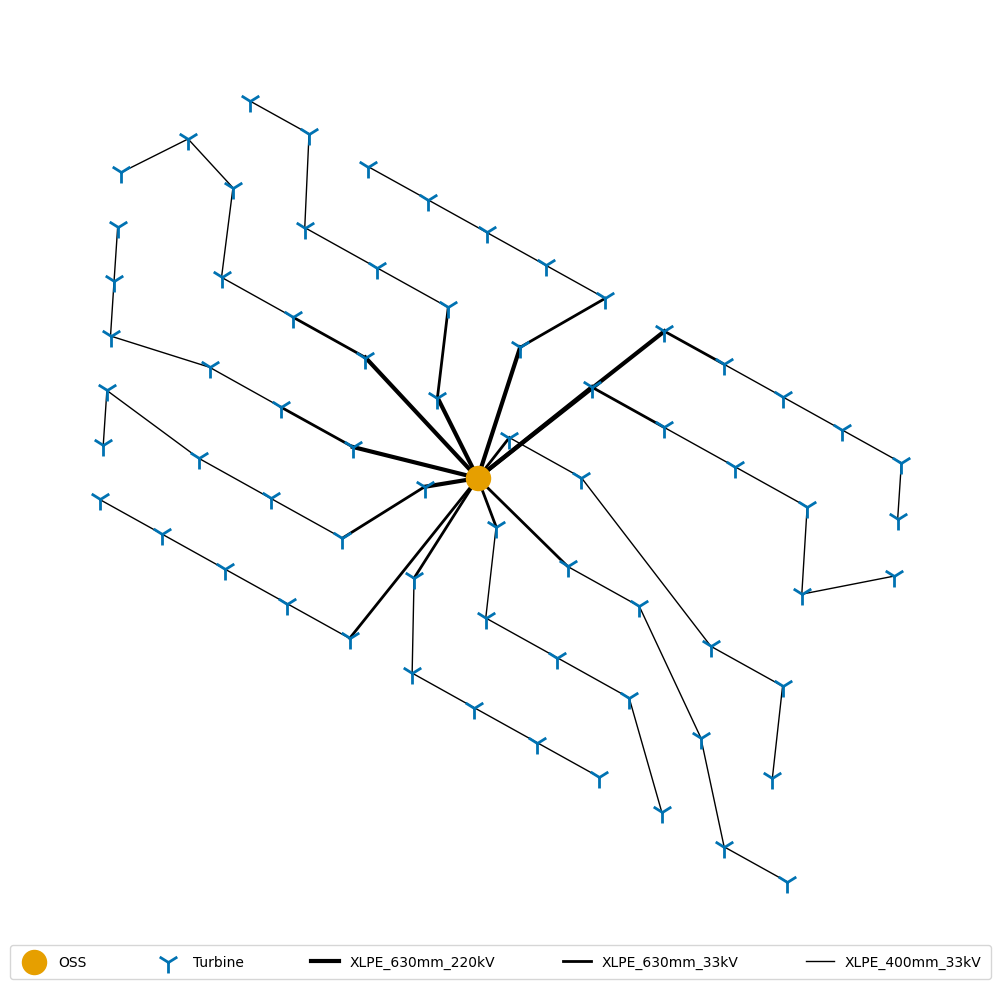
Here the cable length and bury speed are still set to 0 to indicate that they are unknown, which will tell the installation phase to use either ORBIT's defaults or the vessel's settings. Notice that the latitude and longitude here are WGS-84 decimal coordinates.

array.location_data

	id	substation_id	substation_name	substation_latitude	substation_longitude	turbine_name	turbine_latitude	turbine_longitude	string	order	cable_length	bury_speed
0	DAE_A1	DOW_OSS	DOW_OSS	53.2648	1.378767	DAE_A1	53.243950	1.358783	0	0	0.0	0.0
1	DAD_A2	DOW_OSS	DOW_OSS	53.2648	1.378767	DAD_A2	53.248467	1.349033	0	1	0.0	0.0
2	DAC_A3	DOW_OSS	DOW_OSS	53.2648	1.378767	DAC_A3	53.252983	1.339283	0	2	0.0	0.0
3	DAB_A4	DOW_OSS	DOW_OSS	53.2648	1.378767	DAB_A4	53.257500	1.329550	0	3	0.0	0.0
4	DAA_A5	DOW_OSS	DOW_OSS	53.2648	1.378767	DAA_A5	53.262017	1.319800	0	4	0.0	0.0
...	...	...	...	...	...	...	...	...	...	...	...	...
57	DCE_L1	DOW_OSS	DOW_OSS	53.2648	1.378767	DCE_L1	53.251783	1.368833	11	0	0.0	0.0
58	DAF_L2	DOW_OSS	DOW_OSS	53.2648	1.378767	DAF_L2	53.239433	1.368533	11	1	0.0	0.0
59	DAG_L3	DOW_OSS	DOW_OSS	53.2648	1.378767	DAG_L3	53.234917	1.378250	11	2	0.0	0.0
60	DAH_L4	DOW_OSS	DOW_OSS	53.2648	1.378767	DAH_L4	53.230400	1.388000	11	3	0.0	0.0
61	DAJ_L5	DOW_OSS	DOW_OSS	53.2648	1.378767	DAJ_L5	53.225883	1.397750	11	4	0.0	0.0

67 rows × 12 columns

For later comparison, we'll show the cabling costs for the straight-line cabling assumption.

print(f"{'Cable Type':<16}|  {'Cost in USD':>15}")
for cable, cost in array.cost_by_type.items():
    print(f"{cable:<16}| ${cost:>15,.2f}")

print(f"{'Total':<16}| ${array.total_cable_cost:>15,.2f}")

Cable Type      |      Cost in USD
XLPE_400mm_33kV | $  18,701,160.61
XLPE_630mm_33kV | $   8,144,423.11
XLPE_630mm_220kV| $  10,361,949.24
Total           | $  37,207,532.97

Case 3: Distance-based coordinate system

In this case, we will consider each turbine and substation on a distance-based coordinate system where the longitude and latitude are the longitudinal (x direction) and latitudinal (y direction) distances, in kilometers, from a common reference point. We are still using the Dudgeon data, but the distances were computed outside of this example and the details are not be included.

Important

For distance-based coordinate systems, all points should be be positive, meaning the reference point should either be both west and south of the farm itself, or at the west-most and south-most point.

Below, we can see that the input file library/cables/dudgeon_distance_based.csv is still encoded in the exact same manner as Case 2, but latitude and longitude are relative distances and not proper coordinates.

df = pd.read_csv(library_path / "cables/dudgeon_distance_based.csv", index_col=False).fillna("")
df

	id	substation_id	name	longitude	latitude	string	order	cable_length	bury_speed
0	DOW_OSS	DOW_OSS	DOW_OSS	16.229909	35.769173
1	DAE_A1	DOW_OSS	DAE_A1	14.890845	33.450759	0.0	0.0	0.0	0.0
2	DAD_A2	DOW_OSS	DAD_A2	14.237528	33.953026	0.0	1.0	0.0	0.0
3	DAC_A3	DOW_OSS	DAC_A3	13.584211	34.455182	0.0	2.0	0.0	0.0
4	DAB_A4	DOW_OSS	DAB_A4	12.932034	34.957450	0.0	3.0	0.0	0.0
...	...	...	...	...	...	...	...	...	...
63	DCE_L1	DOW_OSS	DCE_L1	15.564263	34.321749	11.0	0.0	0.0	0.0
64	DAF_L2	DOW_OSS	DAF_L2	15.544161	32.948491	11.0	1.0	0.0	0.0
65	DAG_L3	DOW_OSS	DAG_L3	16.195266	32.446335	11.0	2.0	0.0	0.0
66	DAH_L4	DOW_OSS	DAH_L4	16.848583	31.944067	11.0	3.0	0.0	0.0
67	DAJ_L5	DOW_OSS	DAJ_L5	17.501899	31.441800	11.0	4.0	0.0	0.0

68 rows × 9 columns

Using the distance-based location data requires us to set distance to True in the array_system_design section of the configuration. This change is shown below in the library/project/config/example_custom_array_simple_distance_based.yaml configuration.

config = library.extract_library_specs("config", "example_custom_array_simple_distance_based")
pprint(config)

{'array_system_design': {'cables': ['XLPE_400mm_33kV',
                                    'XLPE_630mm_33kV',
                                    'XLPE_630mm_220kV'],
                         'distance': True,
                         'location_data': 'dudgeon_distance_based'},
 'plant': {'layout': 'custom', 'num_turbines': 67},
 'site': {'depth': 20},
 'turbine': 'SWT_6MW_154m_110m'}

Alternatively, we can set the distance=True when calling the CustomArraySystemDesign, however the configuration dictionary's setting will override this input to allow for project-level configurations to run as expected. Below, we can see some of the cable lengths differ slightly due to the methodology of converting the WGS-84coordinates to relative points, however the spacing is maintained, and we can see that this is still the Dudgeon wind farm.

array_distance = CustomArraySystemDesign(config, distance=True)
array_distance.run()
array_distance.plot_array_system(show=True)

UserWarning: /opt/hostedtoolcache/Python/3.13.13/x64/lib/python3.13/site-packages/ORBIT/phases/design/array_system_design.py:1103
Missing data in columns ['cable_length', 'bury_speed']; all values will be calculated.

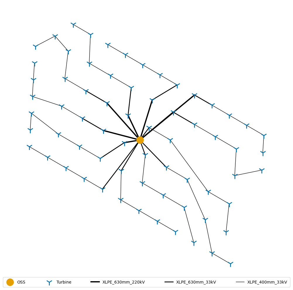
Overall, the cabling cost is highly similar, with the difference being attributed to the method to convert the WGS-84 coordinates to relative coordinates.

print(f"{'Cable Type':<16} | {'Cost in USD (lat,lon)':>20} | {'Cost in USD (dist_lat,dist_lon)':>15}")
for (cable1, cost1), (cable2, cost2) in zip(array.cost_by_type.items(), array_distance.cost_by_type.items()):
    print(f"{cable1:<16} | ${cost1:>20,.2f} | ${cost2:>15,.2f}")

print(f"{'Total':<16} | ${array.total_cable_cost:>20,.2f} | ${array_distance.total_cable_cost:>15,.2f}")

Cable Type       | Cost in USD (lat,lon) | Cost in USD (dist_lat,dist_lon)
XLPE_400mm_33kV  | $       18,701,160.61 | $  18,756,091.16
XLPE_630mm_33kV  | $        8,144,423.11 | $   8,166,522.03
XLPE_630mm_220kV | $       10,361,949.24 | $  10,392,923.05
Total            | $       37,207,532.97 | $  37,315,536.24

Case 4: Site-Wide Cable Length Modifications

To account for exclusion zones from rocky soil or other seabed conditions, we use the average_exclusion_percent input in the array_system_design configuration section. This exclusion will be applied to all cable sections, so it's important to account for this when modeling additional cable lengths.

In the library/project/config/example_custom_array_exclusions.yaml configuration, a 4.8% exclusion is applied to the entire farm. When plotting farms with exclusion zones, they will not be shown since we are not mapping the true cable path, simply the connections between turbines. In this case, we can also a modest increase in cabling costs resulting from the additional cable required to account for the exclusion zones.

config = library.extract_library_specs("config", "example_custom_array_exclusions")
pprint(config)

array_exclusion = CustomArraySystemDesign(config)
array_exclusion.run()

{'array_system_design': {'average_exclusion_percent': 0.05,
                         'cables': ['XLPE_400mm_33kV',
                                    'XLPE_630mm_33kV',
                                    'XLPE_630mm_220kV'],
                         'location_data': 'dudgeon_array'},
 'plant': {'layout': 'custom', 'num_turbines': 67},
 'site': {'depth': 20},
 'turbine': 'SWT_6MW_154m_110m'}

UserWarning: /opt/hostedtoolcache/Python/3.13.13/x64/lib/python3.13/site-packages/ORBIT/phases/design/array_system_design.py:1103
Missing data in columns ['cable_length', 'bury_speed']; all values will be calculated.

print(f"{'Cable Type':<16}|  {'Cost in USD':>15}")
for cable, cost in array_exclusion.cost_by_type.items():
    print(f"{cable:<16}| ${cost:>15,.2f}")

print(f"{'Total':<16}| ${array_exclusion.total_cable_cost:>15,.2f}")

Cable Type      |      Cost in USD
XLPE_400mm_33kV | $  19,601,240.84
XLPE_630mm_33kV | $   8,538,527.60
XLPE_630mm_220kV| $  10,868,096.91
Total           | $  39,007,865.35

Case 5: Custom Cable Lengths

If we look at the map in the Call to Mariners there are different sized exclusions in the cables, so for this example we'll change the distances from Case 4 to have more variation by using the cable_length column of the location_data CSV. In addition, we will utilize the bury_speed column to demonstrate how these columns will be used. Please note this work was performed outside the example, and we will only show the resulting configurations.

For this example, half of the wind farm will have different soil condition, so we will use our proxy: bury_speed by modifying the burial speed to be fast (0.5 km/h) and slow (0.05 km/hr), respectively, to account for sandy soil and rocky soil. The purpose of this is for passing through customized parameters in the design phase to be utilized in the installation phase as will be seen in the final two examples.

config = library.extract_library_specs("config", "example_custom_array_custom")
pprint(config)

array_custom = CustomArraySystemDesign(config)
array_custom.run()

{'array_system_design': {'cables': ['XLPE_400mm_33kV',
                                    'XLPE_630mm_33kV',
                                    'XLPE_630mm_220kV'],
                         'location_data': 'dudgeon_custom'},
 'plant': {'layout': 'custom', 'num_turbines': 67},
 'site': {'depth': 20},
 'turbine': 'SWT_6MW_154m_110m'}

Note that there are now cable lengths defined as well as burial speeds for the installation phase.

array_custom.location_data

	id	substation_id	substation_name	substation_latitude	substation_longitude	turbine_name	turbine_latitude	turbine_longitude	string	order	cable_length	bury_speed
0	DAE_A1	DOW_OSS	DOW_OSS	53.2648	1.378767	DAE_A1	53.243950	1.358783	0	0	3.135279	0.50
1	DAD_A2	DOW_OSS	DOW_OSS	53.2648	1.378767	DAD_A2	53.248467	1.349033	0	1	0.993860	0.50
2	DAC_A3	DOW_OSS	DOW_OSS	53.2648	1.378767	DAC_A3	53.252983	1.339283	0	2	0.993719	0.50
3	DAB_A4	DOW_OSS	DOW_OSS	53.2648	1.378767	DAB_A4	53.257500	1.329550	0	3	0.992699	0.50
4	DAA_A5	DOW_OSS	DOW_OSS	53.2648	1.378767	DAA_A5	53.262017	1.319800	0	4	0.993673	0.50
...	...	...	...	...	...	...	...	...	...	...	...	...
62	DCE_L1	DOW_OSS	DOW_OSS	53.2648	1.378767	DCE_L1	53.251783	1.368833	11	0	1.712822	0.05
63	DAF_L2	DOW_OSS	DOW_OSS	53.2648	1.378767	DAF_L2	53.239433	1.368533	11	1	1.483318	0.05
64	DAG_L3	DOW_OSS	DOW_OSS	53.2648	1.378767	DAG_L3	53.234917	1.378250	11	2	0.901721	0.05
65	DAH_L4	DOW_OSS	DOW_OSS	53.2648	1.378767	DAH_L4	53.230400	1.388000	11	3	0.903679	0.05
66	DAJ_L5	DOW_OSS	DOW_OSS	53.2648	1.378767	DAJ_L5	53.225883	1.397750	11	4	0.903736	0.05

67 rows × 12 columns

Once again, the cabling costs have increased.

print(f"{'Cable Type':<16}|  {'Cost in USD':>15}")
for cable, cost in array_custom.cost_by_type.items():
    print(f"{cable:<16}| ${cost:>15,.2f}")

print(f"{'Total':<16}| ${array_custom.total_cable_cost:>15,.2f}")

Cable Type      |      Cost in USD
XLPE_400mm_33kV | $  20,841,928.36
XLPE_630mm_33kV | $   9,307,325.71
XLPE_630mm_220kV| $  10,158,477.79
Total           | $  40,307,731.86

Incorporating Custom Array Designs Into ProjectManager

Using cases 2, 3, 4, and 5 we will demonstrate the project-wide effects from differing cabling layouts.

Setting Up The Cases

Using the library/project/config/example_array_cable_install.yaml configuration as a base configuration, we'll create a new configuration for each of the cases using each case's design_result as the array_system values.

base_config = library.extract_library_specs("config", "example_array_cable_install")

array_case2 = deepcopy(base_config)
array_case2["array_system"] = array.design_result["array_system"]

array_case3 = deepcopy(base_config)
array_case3["array_system"] = array_distance.design_result["array_system"]

array_case4 = deepcopy(base_config)
array_case4["array_system"] = array_exclusion.design_result["array_system"]

array_case5 = deepcopy(base_config)
array_case5["array_system"] = array_custom.design_result["array_system"]

sim2 = ArrayCableInstallation(array_case2)
sim3 = ArrayCableInstallation(array_case3)
sim4 = ArrayCableInstallation(array_case4)
sim5 = ArrayCableInstallation(array_case5)

Run And Inspect The Simulation Results

We can see that both the installation cost and the time required to complete the installations have all increased here, corresponding to the increased cable lengths and changes to the burial speeds defined above.

names = ("straight-line distance", "distance-based coordinates", "with exclusions", "custom")
simulations = (sim2, sim3, sim4, sim5)

print(f"{'Simulation':<26} | {'Cost (in USD)':>14} | {'Time (in hours)':>16}")
for name, simulation in zip(names, simulations):
    simulation.run()
    cost = simulation.installation_capex
    time = simulation.total_phase_time
    print(f"{name:<26} | ${cost:>13,.2f} | {time:>16,.0f}")

Simulation                 |  Cost (in USD) |  Time (in hours)
straight-line distance     | $24,594,075.16 |            2,372
distance-based coordinates | $24,605,520.50 |            2,373
with exclusions            | $24,784,480.17 |            2,391
custom                     | $31,792,520.58 |            3,088

Incorporating Case 5 Into ProjectManager

We will now incorporate the design settings from Case 5 to demonstrate incorporation of the custom array design tooling into ProjectManager. This example will use the library/project/config/example_custom_array_project_manager.yaml configuration.

config = library.extract_library_specs("config", "example_custom_array_project_manager")
config["array_system_design"]["location_data"] = library.extract_library_specs(
    "cables", config["array_system_design"]["location_data"], file_type="csv"
)
config

{'design_phases': ['CustomArraySystemDesign'],
 'install_phases': ['ArrayCableInstallation'],
 'plant': {'layout': 'custom', 'num_turbines': 67},
 'port': {'monthly_rate': 10000},
 'site': {'depth': 20, 'distance': 50},
 'turbine': 'SWT_6MW_154m_110m',
 'array_system_design': {'cables': ['XLPE_400mm_33kV',
   'XLPE_630mm_33kV',
   'XLPE_630mm_220kV'],
  'location_data':          id substation_id     name   latitude  longitude  string  order  \
  0   DOW_OSS       DOW_OSS  DOW_OSS  53.264800   1.378767     NaN    NaN   
  1    DAE_A1       DOW_OSS   DAE_A1  53.243950   1.358783     0.0    0.0   
  2    DAD_A2       DOW_OSS   DAD_A2  53.248467   1.349033     0.0    1.0   
  3    DAC_A3       DOW_OSS   DAC_A3  53.252983   1.339283     0.0    2.0   
  4    DAB_A4       DOW_OSS   DAB_A4  53.257500   1.329550     0.0    3.0   
  ..      ...           ...      ...        ...        ...     ...    ...   
  63   DCE_L1       DOW_OSS   DCE_L1  53.251783   1.368833    11.0    0.0   
  64   DAF_L2       DOW_OSS   DAF_L2  53.239433   1.368533    11.0    1.0   
  65   DAG_L3       DOW_OSS   DAG_L3  53.234917   1.378250    11.0    2.0   
  66   DAH_L4       DOW_OSS   DAH_L4  53.230400   1.388000    11.0    3.0   
  67   DAJ_L5       DOW_OSS   DAJ_L5  53.225883   1.397750    11.0    4.0   
  
      cable_length  bury_speed  
  0            NaN         NaN  
  1       3.135279        0.50  
  2       0.993860        0.50  
  3       0.993719        0.50  
  4       0.992699        0.50  
  ..           ...         ...  
  63      1.712822        0.05  
  64      1.483318        0.05  
  65      0.901721        0.05  
  66      0.903679        0.05  
  67      0.903736        0.05  
  
  [68 rows x 9 columns],
  'distance': False},
 'array_cable_install_vessel': 'example_cable_lay_vessel',
 'array_cable_bury_vessel': 'example_cable_lay_vessel'}

Below, we can see that the results coming from the ProjectManager are the same as the additive results of running each phase separately.

project = ProjectManager(config)
project.run()

total = array_custom.total_cable_cost + sim5.installation_capex
print(f"Custom Design        | ${array_custom.total_cable_cost:>13,.2f}")
print(f"Custom Installation  | ${sim5.installation_capex:>13,.2f}")
print(f"Total Custom Cost    | ${total:>13,.2f}")
print(f"Project Manager Cost | ${project.bos_capex:>13,.2f}")

Custom Design        | $40,307,731.86
Custom Installation  | $31,792,520.58
Total Custom Cost    | $72,100,252.44
Project Manager Cost | $72,100,252.44