HVAC vs HVDC Systems

Technology decisions have an impact on a wind project's CapEx. This example will provide a basic setup to compare how different project sizes, export cable types (HVDC or HVDC), distances to shore, and etc. effect project costs. Instead of other guides' approach of using the ExportSystemDesign, this will highlight the use of the ElectricalDesign model that co-designs the substation and export cabling system.

from copy import deepcopy

import numpy as np
import pandas as pd
import matplotlib.pyplot as plt
from matplotlib.ticker import StrMethodFormatter

from ORBIT.phases.design import ElectricalDesign
from ORBIT import ProjectManager, ParametricManager

# Apply thousands separators and no decimals to floats
pd.options.display.float_format = '{:,.0f}'.format

Setup The Models

Here we will setup a base configuration for use with ProjectManager plus additional configurations for running in the ParametricManager to look at the cost tradeoffs in export cable types depending on project size. Config must include all required variables except those you plan to vary. In this example, we will be manually vary the cable type and then use the ParametricManager to vary cable type and plant capacity.

base_config = {
    "export_cable_install_vessel": "example_cable_lay_vessel",
    "site": {
        "distance": 100,
        "depth": 20,
        "distance_to_landfall": 80,
    },
    "plant": {
        "capacity": 1000,
    },
    "turbine": "12MW_generic",
    "oss_install_vessel": "example_heavy_lift_vessel",
    "feeder": "future_feeder",
    "design_phases": [
        "ElectricalDesign",
    ],
    "install_phases": [
        "ExportCableInstallation",
        "OffshoreSubstationInstallation",
    ],
}

Now we can create an HVAC and HVDC variation of the base_config

hvac_config = deepcopy(base_config)
hvac_config["export_system_design"] = {"cables": "XLPE_1000mm_220kV"}

hvdc_config = deepcopy(base_config)
hvdc_config["export_system_design"] = {"cables": "HVDC_2000mm_320kV"}


hvac_project = ProjectManager(hvac_config)
hvac_project.run()

hvdc_project = ProjectManager(hvdc_config)
hvdc_project.run()

ORBIT library intialized at '/opt/hostedtoolcache/Python/3.13.13/x64/lib/python3.13/site-packages/library'
OffshoreSubstationInstallation:
	 Warning: 'Feeder 0' Cargo Mass Capacity Exceeded
OffshoreSubstationInstallation:
	 Warning: 'Feeder 0' Cargo Mass Capacity Exceeded

Compare the Results

print(f"HVAC CapEx per kW: ${hvac_project.total_capex_per_kw:,.2f} ")
print(f"HVDC CapEx per kW: ${hvdc_project.total_capex_per_kw:,.2f} ")

HVAC CapEx per kW: $3,248.11 
HVDC CapEx per kW: $3,453.34

capex_df = (
    pd.DataFrame(
        [*hvac_project.capex_breakdown.items()],
        columns=["Category", "HVAC CapEx"]
    ).set_index("Category")
    .join(
        pd.DataFrame(
            [*hvdc_project.capex_breakdown.items()],
            columns=["Category", "HVDC CapEx"]
        ).set_index("Category")
    )
)
capex_df

	HVAC CapEx	HVDC CapEx
Category
Export System	498,419,536	149,436,000
Offshore Substation	249,766,921	795,031,033
Export System Installation	75,818,732	20,475,204
Offshore Substation Installation	3,861,208	3,861,208
Onshore Substation	200,437,705	254,763,736
Turbine	1,310,400,000	1,310,400,000
Soft	554,406,805	564,374,443
Project	355,000,000	355,000,000

Setup The Parametric Runs

From the two base cases above, we see that HVDC cables are more cost effective than HVAC at roughly 30% of the HVAC cable costs. However, the offshore substation (OSS) is over three times the cost of an HVAC OSS. To compare this sensitivity and see if there is an point that these technologies cross we'll use the ParametricManager and sweep each cable for a range of plant capacities.

capacity_range = np.arange(100, 4100, 100)
parameters = {
    "export_system_design.cables": ["XLPE_1000mm_220kV", "HVDC_2000mm_320kV"],
    "plant.capacity": capacity_range,
}

results = {
    "cable_cost": lambda run: run.total_cable_cost,
    "oss_cost": lambda run: run.total_substation_cost,
    "num_cables": lambda run: run.num_cables,
    "num_substations": lambda run: run.num_substations,
}

parametric = ParametricManager(
    base_config, parameters, results, module=ElectricalDesign, product=True
)
parametric.run()

Compare the Cost vs Capacity Trade Off

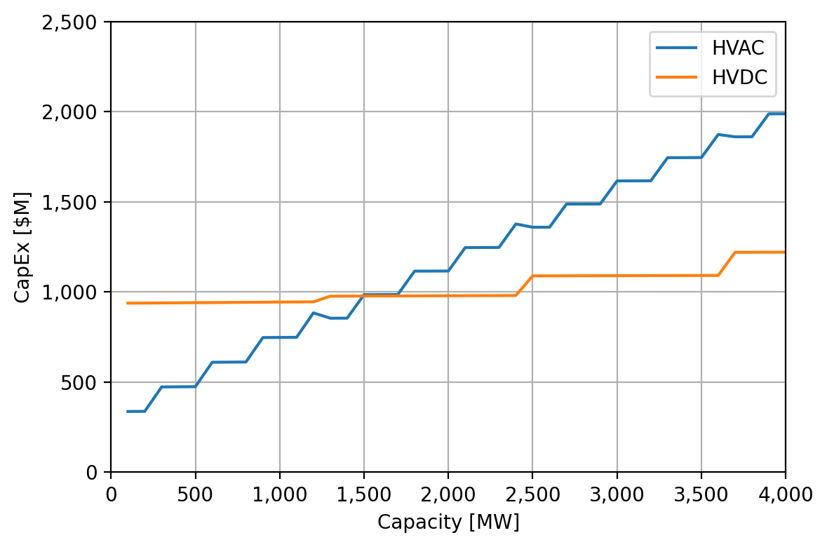
The inflection point of the below graph shows that for projects with about 100 km of export cabling that 1,400 MW of capacity is the point at which HVDC becomes more cost effective than HVAC.

Not shown in this example, but generally for near shore projects, HVAC will be more cost effective, but as the cabling length grows, the project size required for the economics to favor HVDC shrinks.

df = pd.DataFrame(parametric.results)

hvac_df = df[df["export_system_design.cables.XLPE_1000mm_220kV.name"] == "XLPE_1000mm_220kV"]
hvdc_df = df[df["export_system_design.cables.HVDC_2000mm_320kV.name"] == "HVDC_2000mm_320kV"]

fig = plt.figure(figsize=(6,4), dpi=200)
ax = fig.subplots(1)

ax.plot(
    hvac_df["plant.capacity"],
    (hvac_df["cable_cost"] + hvac_df["oss_cost"]) / 1e6,
    label="HVAC"
)

ax.plot(
    hvdc_df["plant.capacity"],
    (hvdc_df["cable_cost"] + hvdc_df["oss_cost"]) / 1e6,
    label="HVDC",
)

ax.set_xlim(0, capacity_range.max())
ax.set_ylim(0, 2500)

ax.xaxis.set_major_formatter(StrMethodFormatter("{x:,.0f}"))
ax.yaxis.set_major_formatter(StrMethodFormatter("{x:,.0f}"))

ax.set_ylabel("CapEx [$M]")
ax.set_xlabel("Capacity [MW]")
ax.legend()
ax.grid()

fig.tight_layout()

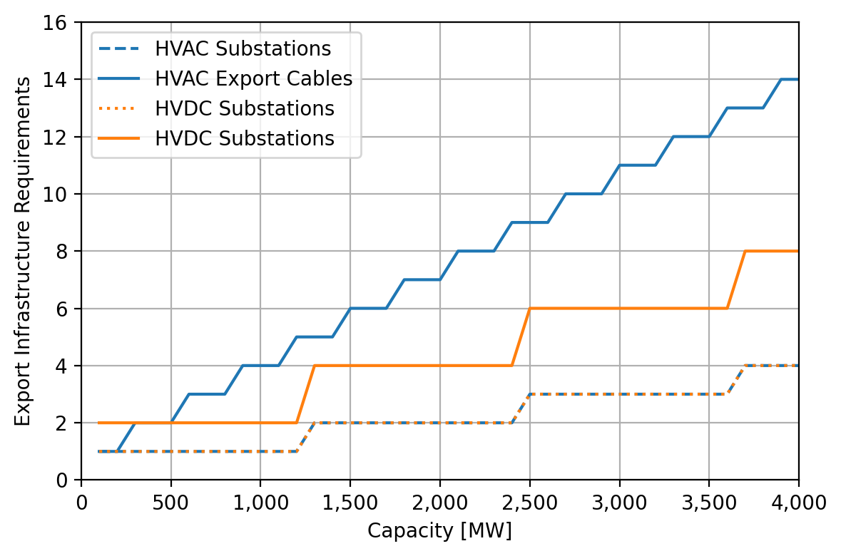
Comparing the below figure to the CapEx figure above, highlights that CapEx increases for the HVDC system correspond to an increase in the number of substations (each requires a single cable), whereas for HVAC system, these increases primarily correspond to an increase in the number of export cables with a smaller increase stemming from the substation requirements.

fig = plt.figure(figsize=(6,4), dpi=200)
ax = fig.subplots(1)

ax.plot(hvac_df["plant.capacity"], hvac_df["num_substations"], c="tab:blue", ls="--", label="HVAC Substations")
ax.plot(hvac_df["plant.capacity"], hvac_df["num_cables"], c="tab:blue", ls="-", label="HVAC Export Cables")
ax.plot(hvdc_df["plant.capacity"], hvdc_df["num_substations"], c="tab:orange", ls="dotted", label="HVDC Substations")
ax.plot(hvdc_df["plant.capacity"], hvdc_df["num_cables"], c="tab:orange", ls="-", label="HVDC Substations")

ax.set_xlim(0, capacity_range.max())
ax.set_ylim(0, 16)

ax.xaxis.set_major_formatter(StrMethodFormatter("{x:,.0f}"))
ax.yaxis.set_major_formatter(StrMethodFormatter("{x:,.0f}"))

ax.set_xlabel("Capacity [MW]")
ax.set_ylabel("Export Infrastructure Requirements")
ax.legend()
ax.grid()

fig.tight_layout()