Modeling Supply Chains

In this example we will model the effects of the supply chain on substructure fabrication on jacket-pile installations. For this example we will consider the following three cases:

1. Jacket installations with unlimited port storage.

2. Insufficient jacket fabrication to match installation rates.

3. Increased jacket fabrication to keep pace with installation rates.

from copy import deepcopy
from pathlib import Path

import pandas as pd
import matplotlib.pyplot as plt

from ORBIT import ProjectManager, load_config
from ORBIT.phases.install import MonopileInstallation, JacketInstallation

# Set the example path for use in the docs and standalone examples usage
here = Path(".").resolve()
match here.stem:
    case "examples":
        example_path = here
    case "topical_guides":
        example_path = here.parents[1] / "examples"
    case "ORBIT":
        example_path = here / "examples"
    case _:
        msg = "Please manually change `example_path` if running in a custom location."
        raise FileNotFoundError(msg)

weather = pd.read_csv(
    example_path / "data/example_weather.csv", parse_dates=["datetime"]
).set_index("datetime")

UserWarning: /tmp/ipykernel_2572/3771038313.py:23
Could not infer format, so each element will be parsed individually, falling back to `dateutil`. To ensure parsing is consistent and as-expected, please specify a format.

Preparing The Cases

Here, we will load the examples/configs/example_fixed_project.yaml configuration and modify it to run a jacket installation process. Please note that there is no jacket design model in ORBIT, so we must provide the basic jacket parameterizations for the design result.

base_jacket_config = load_config(example_path / "configs/example_fixed_project.yaml")
base_jacket_config["jacket"] = {
    "diameter": 10,
    "height": 100,
    "length": 100,
    "mass": 100,
    "deck_space": 100,
    "unit_cost": 1e6
}

slow_prod_config = deepcopy(base_jacket_config)
slow_prod_config["jacket_supply_chain"] = {
    "enabled": True,
    "substructure_delivery_time": 500,
    "num_substructures_delivered": 2,
}

increased_prod_config = deepcopy(base_jacket_config)
increased_prod_config["jacket_supply_chain"] = {
    "enabled": True,
    "substructure_delivery_time": 250,
    "num_substructures_delivered": 2,
}

case1_project = JacketInstallation(base_jacket_config, weather=weather)
case2_project = JacketInstallation(slow_prod_config, weather=weather)
case3_project = JacketInstallation(increased_prod_config, weather=weather)

case1_project.run()
case2_project.run()
case3_project.run()

ORBIT library intialized at '/opt/hostedtoolcache/Python/3.13.13/x64/lib/python3.13/site-packages/library'

Comparing Results

Installation Time

print(f"Case 1 Installation Time: {case1_project.total_phase_time / 24:.1f} days")
print(f"Case 2 Installation Time: {case2_project.total_phase_time / 24:.1f} days")
print(f"Case 3 Installation Time: {case3_project.total_phase_time / 24:.1f} days")

Case 1 Installation Time: 319.8 days
Case 2 Installation Time: 540.9 days
Case 3 Installation Time: 327.1 days

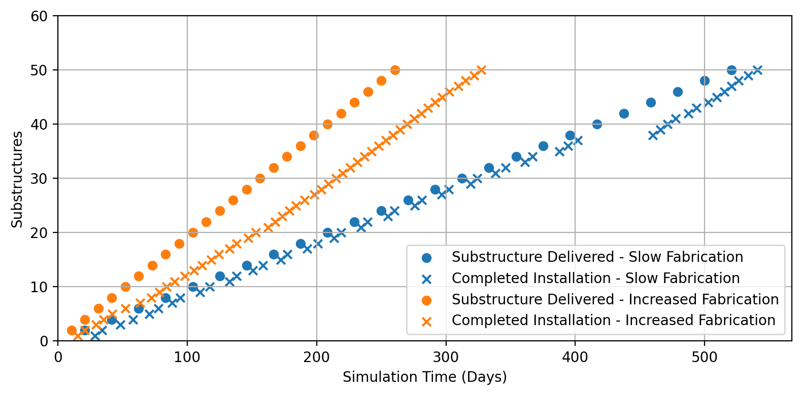
Installation Timing

Below, we plot the timing of jacket deliveries and their subsequent installations without considering vessel logistic delays. Note the inclement weather around the 400th day of Case 2's installation simulation.

case2_df = pd.DataFrame(case2_project.env.actions)
case2_deliveries = case2_df.loc[case2_df["action"].str.contains("Delivered"), ["action", "time"]]
case2_deliveries["number"] = case2_deliveries["action"].str.split(" ").str[1].astype(int)

case2_installs = case2_df.loc[case2_df["action"].str.contains("Grout Jacket"), ["action", "time"]]
case2_installs["number"] = 1

case2_deliveries.time /= 24.0
case2_installs.time /= 24.0


case3_df = pd.DataFrame(case3_project.env.actions)
case3_deliveries = case3_df.loc[case3_df["action"].str.contains("Delivered"), ["action", "time"]]
case3_deliveries["number"] = case3_deliveries["action"].str.split(" ").str[1].astype(int)

case3_installs = case3_df.loc[case3_df["action"].str.contains("Grout Jacket"), ["action", "time"]]
case3_installs["number"] = 1

case3_deliveries.time /= 24.0
case3_installs.time /= 24.0

fig = plt.figure(figsize=(8,4), dpi=200)
ax = fig.add_subplot(111)

ax.scatter(
    case2_deliveries["time"],
    case2_deliveries["number"].cumsum(),
    marker="o",
    c="tab:blue",
    label="Substructure Delivered - Slow Fabrication"
)
ax.scatter(
    case2_installs["time"],
    case2_installs["number"].cumsum(),
    marker="x",
    c="tab:blue",
    label="Completed Installation - Slow Fabrication"
)

ax.scatter(
    case3_deliveries["time"],
    case3_deliveries["number"].cumsum(),
    marker="o",
    c="tab:orange",
    label="Substructure Delivered - Increased Fabrication"
)
ax.scatter(
    case3_installs["time"],
    case3_installs["number"].cumsum(),
    marker="x",
    c="tab:orange",
    label="Completed Installation - Increased Fabrication"
)

ax.set_xlim(0, ax.get_xlim()[1])
ax.set_ylim(0, 60)

ax.set_xlabel("Simulation Time (Days)")
ax.set_ylabel("Substructures")

ax.legend()
ax.grid()
fig.tight_layout()

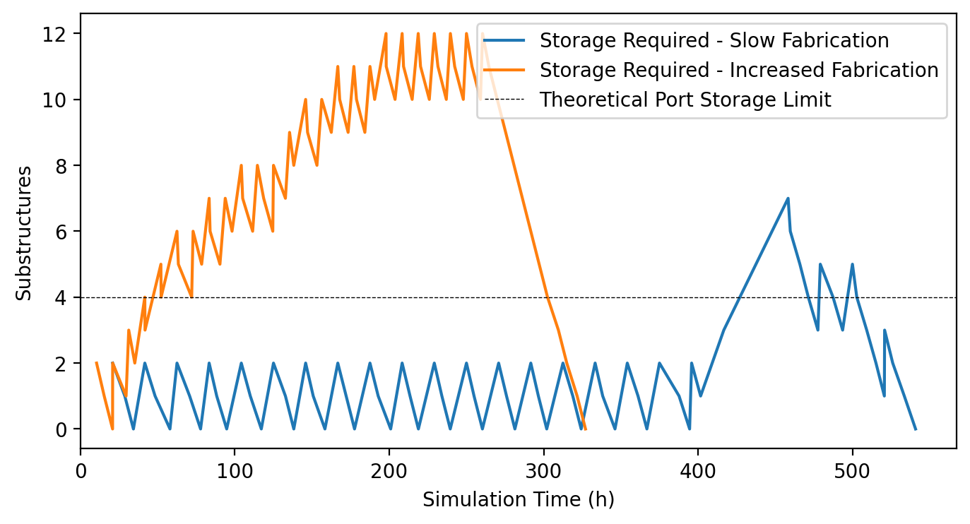
Port Storage

fig = plt.figure(figsize=(8,4), dpi=200)
ax = fig.add_subplot(111)

case2_installs_neg = case2_installs.copy()
case2_installs_neg["number"] *= -1
case2_total = pd.concat([case2_deliveries, case2_installs_neg]).sort_values("time")
case2_total["storage"] = case2_total["number"].cumsum()

case3_installs_neg = case3_installs.copy()
case3_installs_neg["number"] *= -1
case3_total = pd.concat([case3_deliveries, case3_installs_neg]).sort_values("time")
case3_total["storage"] = case3_total["number"].cumsum()

ax.plot(
  case2_total["time"],
  case2_total["storage"],
  label="Storage Required - Slow Fabrication"
)
ax.plot(
  case3_total["time"],
  case3_total["storage"],
  label="Storage Required - Increased Fabrication"
)

ax.set_xlim(0, ax.get_xlim()[1])
# ax.set_ylim(0, 5)

ax.axhline(4, ls="--", lw=0.5, c="k", label="Theoretical Port Storage Limit")

ax.set_xlabel("Simulation Time (h)")
ax.set_ylabel("Substructures")

ax.legend()
fig.show()